
A model developed in one context (e.g. a place, population, and time) may be powerful and highly accurate when used in that context, but inaccurate, misleading, or biased in a different context. When an analytical system is used in a context to which it is poorly suited we call this an error of applicability. The data validation tools available with our tdda library are a key way of protecting against this failure mode, though there are other practices that can also help, as discussed below.
TDDA’s approach to data validation is based on a pair of capabilities in the software.
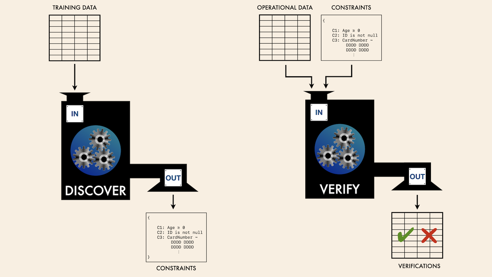
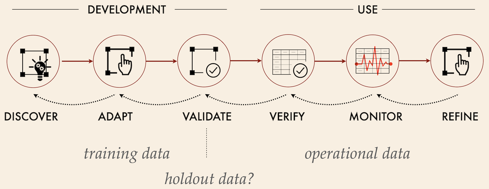
First, constraints are generated from known-good or believed-to-be-good data, which plays the role of training data. These constraints characterize the data fairly tightly. The constraints generated can then be used to validate new data, confirming that the new data has the same characteristics as the training data. Ideally, the constraints are not used blindly, but are first examined and refined, and the system is monitored in use and further adjustments are made as false positives and false negatives appear, which is always likely.
This adaptation process is shown below.
In the context of detecting errors of applicability and data drift, both inputs and outputs should be validated, both at record level and whole dataset/distribution level.
As well as detecting processes that are performing poorly, these approaches can help to detect algorithmic bias, which in addition to being intrinsic harmful and undesirable, also constitutes legal-, compliance-, and reputational risk.
Abstract and Concrete Decisions. When developing analyses, whether this is by building models or simply taking measurements and reporting, many decisions always get taken in light of the data used in development. As a simple example, a variable may be divided into deciles. The boundaries between deciles are (by definition) a function of the development data—perhaps the boundary between the first and second decile comes out at 1.2. On that development data, there is no practical difference between specifying that boundary 1.2 or “the tenth percentile value“, but when the equivalent breakdown is applied to different data, the first decile might be at a completely different values (perhaps 1.8). We call specifications based on fixed values like 1.2 concrete specifications, while data-dependent values like “the tenth percentile value” are abstract specifications.
Whether presenting a table, drawing a graph, or preprocessing data for a model, the choice as to whether to use concrete or abstract specifications is subtle and there is not a one-size-fits-all answer to which is more appropriate. In most cases, when deploying a model, concrete specifications are the better choice, because they bake in more of the assumptions of the modelling and make it more likely that outputs have the same meaning and that drift can be detected. But this is not universal. Abstract specification are more adaptive, and in some kinds of modelling it is relative rather than absolute values that are more important; in these cases, careful choices of abstract specifications may in fact be appropriate. In reporting, either can be appropriate, but when designing the reports, it is important to be deliberate about the choices made and to understand and clarify the implications of those choices.
A special case of abstract and concrete representation is time, where the considerations are different. At a given time, people’s birthdays and ages are perfectly linearly (anti-)correlated and have the same information content. Most predictive modelling is based on moveable observation windows that use relative time (here, ages) and can be moved forward when progressing from older training data to newer “longitudinal” validation data, and then as the model is used over time. With all such training, models are built using outcome periods in the more recent past and observations from the more distant past, and it is critically important that the training data genuinely involves predictors (independent variables) in the state they genuinely were at the time they represent in the training data, and are not contaminated with more recent information that was not, in reality, available at the end of the training window’s observation period. This failure mode is one of the most common, and something we encounter with monotonous regularity when working with clients. Two indicators that such contamination may be occurring are:
The surest way to avoid this form of contamination is to keep dated immutable snapshots of data likely to be used in model development, and to be certain only to use data as it was at the relevant cut-off points when developing models.
Notwithstanding these observations, relative time is not always the most useful time as cohort effects also exist. A cohort is a group of people for whom a fixed reference data is important: this can be a cohort based on date of birth, or something not directly age based such as date of recruitment. Generations (“baby boomers”, “Generation X” etc.) are one example of birth-based cohorts, and in some situations these are more important predictors than age per se, meaning that absolute dates might be useful in models. Similarly, it may be that customer onboarding processes have changed significantly over time, so that when customers recruited at different specific times behave differently.
Sometimes cohort effects show up through other variables. In a recent customer engagement, the presence of nulls in a field turned out to be highly predictive (indicating that these were x-nulls rather than μ-nulls). After some digging, it transpired that the values were null for older entities where data was not available, and that including the absolute date was a more powerful predictor. (In this particular case, the client had imputed values for the missing data, which made this significantly harder to detect, and emphasising the importance of understanding the causes of null values, and whether or not they are missing completely at random (MCAR)). When they are not, they may contain information, should not be imputed, and might be useful as predictors.
Much more detail on all the topics discussed here is available in the TDDA Book, with Chapter 2 introducing data validation and Chapters 5 to Chapter 7 providing detailed guides, examples and discussions of that topic. Chapter 17 discusses Errors of Applicability more specifically, along with Errors of Judgement.
If your data analysis processes and pipelines are not working as you need them to, get in touch. We have a long track record of helping companies to diagnose and remedy problems such as those discussed here, and can help train teams to reduce the likelihood, frequency, and severity of these problems with timely detection. This may include working with data engineering and data governance teams to help with good data versioning and collection, understanding lineage, and helping to provide a solid foundation on which analytical teams can build more productively.